差分进化算法

差分进化算法（Differential Evolution，DE）是一种基于向量的元启发式算法，具有良好的收敛性。DE 变体有很多，并且已经在广泛的学科中得到应用。这里简要介绍基本差分进化及其主要实现细节和变体。讨论了种群方差的基本收敛性。

简介

差分进化（Differential Evolution，DE）是在 1996 年和 1997 年 R.Storn 和 K.Price 的论文中发展起来的[7, 8]。DE 是一种基于向量的元启发式算法，由于其交叉和变异的特点，与模式搜索和遗传算法有一定的相似性。实际上，DE 算法可以看作是对具有显式更新方程遗传算法的进一步发展，使理论分析成为可能。DE 算法是一种具有自组织倾向的随机搜索算法，不使用导数信息。因此，它是一种基于群体的、无导数的方法。此外，DE 使用实数作为解串，因此不需要编码和解码。

与遗传算法一样，d 维搜索空间中的设计参数被表示为向量，并且各种遗传算子对它们的位串进行操作。然而，与遗传算法不同，差分进化对每个组件（或解的每个维度）执行操作。几乎所有的事情都是用向量来完成的。例如，在遗传算法中，突变是在染色体的一个位点或多个位点进行的，而在差异进化中，使用两个随机选择的群体向量的差异向量来对现有向量进行调整。从实现的角度来看，这种向量化突变可以看作是一种更有效的方法。这种扰动是在每个群体向量上进行的，因此可以预期效率更高。类似地，交叉也是基于向量的染色体或向量段的分支交换。

除了使用变异和交叉作为差分算子外，DE 还具有显式的更新方程。这也使得实现和设计新的变体变得简单明了。

差分进化

对于具有 d 个参数的 d 维优化问题，首先生成具有 n 个解向量的种群。我们有 $x_i$，其中 $i=1, 2,..., n$。对第 t 代的解 $x_i$，我们使用常规符号记为：

$$x_i^t = (x_{1,i}^t, x_{2,i}^t, … , x_{d, i}^t), \tag 1$$

其由 d 维空间中的 d 分量组成。这种向量可以被认为是染色体或基因组。

差分进化包括三个主要步骤：变异、交叉和选择。

通过变异方案进行变异。对于第 t 代的每个向量 $x_i$，我们首先随机选择三个不同向量 $x_p$、$x_q$ 和 $x_r$（参见
图 1），然后我们通过变异方案产生变异个体（donor vector）

$$v_i^{t+1} = x_p^t + F(x_q^t - x_r^t), \tag 2$$

其中 $F \in [0, 2]$ 是一个参数，通常称为差分权重（ differential weight）。这要求种群规模的最小值为 $n \ge 4$。原则上，$F \in [0, 2]$，但实际上，$F \in [0, 1]$ 的方案更有效和稳定。事实上，几乎所有的文献中都使用$F \in (0, 1)$。

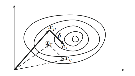
Figure 1 Schematic representation of mutation vectors in differential evolution with movement $\delta=F(x_q - x_r)$.

从图 1 可以看出，向量 $x_p$ 的扰动 $\delta=F(x_q - x_r)$ 用于产生变异个体 $v_i$，并且这种扰动是定向的（directed）。

交叉由交叉参数 $Cr \in [0, 1]$ 控制，控制交叉的速率或概率。实际的交叉可以用两种方式进行：二项式（binomial）和指数式（exponential）。二项式方案对 d 个分量中的每一个分量都进行交叉。通过生成服从均匀分布的随机数 $r_i \in [0, 1]$，$v_i$ 的第 j 个分量被表示为

$$
u_{j, i}^{t+1} =
\begin{cases}
v_{j, i} & \text{if $r_i \le C_r$}, \
x_{j, i}^t & \text{otherwise},
\end{cases}
j = 1, 2, … , d.
\tag 3
$$

这样，可以随机地决定是否与变异个体交换某一分量。

在指数方案中，选择变异个体的一段，且该段以具有随机长度为 L 的随机整数 k 开始，该随机整数 k 可以包含多个分量。在数学上，这是随机选择 $k \in [0, d-1]$ 和 $L \in [1, d]$，我们有

$$
u_{j, i}^{t+1} =
\begin{cases}
v_{j, i}^t & \text{for $j=k,…,k-L+1 \in [1, d]$}, \
x_{j, i}^t & \text{otherwise}.
\end{cases}
\tag 4
$$

由于二项式更易于实现，因此我们将在实现中使用二项式交叉。

选择基本上与遗传算法中使用的相同。我们选择适者（对于最小化问题，选择最小目标函数值）。因此，我们有

$$
x_i^{t=1} =
\begin{cases}
u_i^{t+1} & \text{if $f(u_i^{t+1}) \le f(x_i^t)$}, \
x_i^t & \text{otherwise}.
\end{cases}
\tag 5
$$

在图 2 所示的伪代码中可以看到所有三个组件。这里值得指出的是，使用 J 是为了确保 $v_i^{t+1} \neq x_i^t$，这可以增加进化或探索效率。整体搜索效率由两个参数控制：差分权重 F 和交叉概率 Cr。

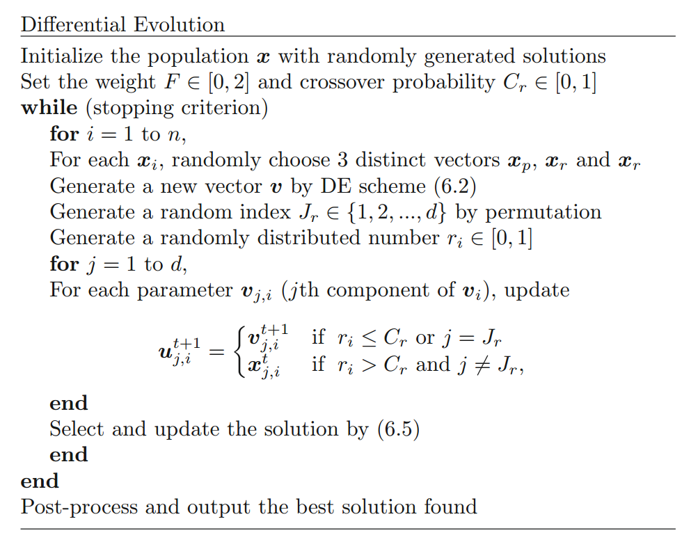
Figure 2 Pseudo code of differential evolution.

算法变体

大多数研究集中在选择 F、Cr 和 n 以及式 2 的修改。事实上，在生成变异向量时，我们可以使用许多不同的方式来形成式 2，并且这产生了方案的命名约定：DE/x/y/z，其中 x 是变异方案（rand 或 best），y 是差分向量的数量，z 是交叉方案（bin 或 exp）。因此，DE/Rand/1/* 意味着该基本 DE 方案使用随机变异、一个差分向量以及二项式或指数交叉。

基本 DE/Rand/1/Bin 方案由式 2 给出。亦即：

$$v_i^{t+1} = x_p^t + F(x_q^t - x_r^t), \tag 6$$

如果我们用当前最佳 $x_{best}$ 替换 $x_p^t$，我们就有所谓的 DE/Best/1/Bin 方案，

$$v_i^{t+1} = x_{best}^t + F(x_q^t - x_r^t). \tag 7$$

我们没有理由不使用三个以上不同的向量。如果我们使用四个不同的向量加上当前的最佳向量，我们就有 DE/Best/2/Bin 方案

$$v_i^{t+1} = x_{best}^t + F(x_{k1}^t + x_{k2}^t - x_{k3}^t - x_{k4}^t). \tag 8$$

此外，如果我们使用 5 个不同的向量，那么我们有 DE/Rand/2/Bin 方案

$$v_i^{t+1} = x_{k1}^t + F_1(x_{k2}^t - x_{k3}^t) + F_2(x_{k4}^t - x_{k5}^t), \tag 9$$

其中 $F_1$ 和 $F_2$ 是取值在 [0, 1] 之间的差分权重。显然，为了简单起见，我们也可以取 $F_1 = F_2 = F$。

遵循类似的策略，我们可以设计各种方案。 例如，这些变体可以用通用形式写成

$$v_i^{t+1} = x_{k1}^t + \sum_{s=1}^m F_s \cdot (x_{k2(s)}^t - x_{k3(s)}^t), \tag {10}$$

其中 $m = 1,2,3,...$，$F_s(s = 1,...,m)$ 为缩放参数。在右侧涉及的向量数为 2m+1。在前面的变体中，m=1 和 m=2 在文献 [9, 14] 有使用。

另一方面，另一种类型的变体使用另外的影响参数 $\lambda \in (0, 1)$。例如 DE/rand-to-best/1/* 变体可以写成

$$v_i^{t+1} = \lambda x_{best}^t + (1 - \lambda)x_{k1}^t + F(x_{k2}^t - x_{k3}^t), \tag {11}$$

它引入了一个额外的参数 $\lambda$。这种类型的变体也可以用一种通用的形式写成：

$$v_i^{t+1} = \lambda x_{best}^t + (1 - \lambda)x_{k1}^t + F \sum_{s=1}^m (x_{k2(s)}^t - x_{k3(s)}^t). \tag {12}$$

事实上，已经有超过 10 个不同的方案，具体请参看 Price 等人的文献 [9]。

还有其他一些很好的 DE 变体，包括 Brest 等人的差分进化中的自适应控制参数（jDE）[2]，自适应 DE（SaDE）[6]，使用鹰策略的 DE [11]。

多目标变体也存在。有关详细的综述，请参阅 Das 和 Suganthan [4] 或 Chakraborty [3]。

参数的选择

参数的选择很重要。经验观察和研究都表明参数值应该进行微调 [4, 5, 9]。

缩放因子 F 是最敏感的因子。尽管 $F \in [0, 1]$ 在理论上是可以接受的，但 $F \in (0, 1)$ 在实践中更有效。事实上，$F \in [0.4, 0.95]$ 是一个很好的范围，首选可以是 $F \in [0.7, 0.9]$。

交叉参数 $C_r \in [0.1, 0.8]$ 似乎是一个很好的范围，首选可以使用 $C_r = 0.5$。

建议种群规模 n 应取决于问题的维数 d。也就是说，n = 5d 到 10d。由于种群规模可能很大，因此这可能对于高维问题来说是一个缺点。但是，没有理由不先尝试固定值（比如 n = 40 或 100）。

收敛性分析

文献 [4,5,10,12-14] 对收敛特性和差分进化的参数敏感性进行了较为广泛的研究。例如，已经观察到 DE 的性能对缩放因子 F 比 Cr 敏感。又如，Xue 等人 [10] 以式 12 的形式分析了一般变体。得出结论

$$2mF^2 + (1 - \lambda)^2 \gt 1, \lambda \in (0, 1). \tag {13}$$

他们还指出，λ 应该相当大，以便更好地收敛。

本节其余部分的结果主要基于 Zaharie 的研究 [13, 14]。避免任何基于群体的算法早熟收敛的条件之一是保持群体中的高度多样性 [1]。任何 DE 变体的方差可以使用种群 $P = \{P_1, P_2, ..., P_n\}$ 的 component-based 期望方差 $E(var(P))$ 来计算。因为我们前面提到的所有变量都是线性的，因此 DE 的期望方差线性依赖于当前种群 $X = (x_1, ..., X_n)$ 的方差。即

$$E(var(P)) = c , var(X), \tag {14}$$

其中 c 是常数。

对于基本的 DE/rand/1/* 方案，Zaharie 计算了无选择时种群的方差，得到

$$E(var(P)) = (1 + 2p_mF^2 - \frac{p_m(2 - p_m)}{n})var(X), \tag {15}$$

其中 $p_m$ 是与交叉参数 $C_r$ 相关的变异概率

$$
p_m =
\begin{cases}
C_r(1 - \frac 1d) + \frac 1d & \text{(binomial crossover)}, \
\frac{1 - C_r^d}{d(1 - C_r)} & \text{(exponential crossover)}.
\end{cases}
\tag {16}
$$

如果初始种群为 $X^{(t=0)} = X(0)$，则第 t 代/迭代后的种群方差变为

$$var(P) = (1 + 2F^2p_m - \frac{p_m(2-p_m)}{n})^tvar(X(0)). \tag {17}$$

这定义了 F 的临界值

$$1 + 2F^2p_m - \frac{p_m(2 - p_m)}{n} = 1, \tag {18}$$

这使得

$$F_c = \sqrt{\frac{(2 - p_m)}{n}}. \tag {19}$$

因此，如果 F < Fc，则群体方差降低，如果 F > Fc，则群体方差增加。显然，当 F = Fc 时，群体方差将保持不变。

例如，对于二项式交叉 Cr = 0.5，d = 10 情况下，我们有

$$p_m = C_r (1 - \frac 1d) + \frac 1d = 0.5 \times (1 - \frac{1}{10}) + \frac{1}{10} = 0.55. \tag {20}$$

经验观察表明 $F \in [0.4, 0.95]$，首选 F = 0.9 [4, 5, 9]。或者，对于给定的 $p_m$，我们可以估算 Cr 值

$$C_r = \frac {(p_m - \frac 1d)}{(1 - \frac 1d)}. \tag {21}$$

所以，对于适中的 $p_m = 0.5,\quad d=10$，我们有

$$C_r = \frac{(0.2 - 1/10)}{(1 - 1/10)} \approx 0.44. \tag {22}$$

有趣的是，当 $d \to \infty$ 时，$C_r \to p_m$。

显然，这些结果对于基本的 DE/Rand/1/* 是有效的。对于其他变体，公式是相似的，其中一些修改包括参数 λ。

这些理论结果意味着当 var(P) 减小时，DE 算法正在收敛。换句话说，当 $var(P) \to 0$ 时，算法已经收敛。然而，这种收敛可能为时过早，因为收敛的状态可能不是问题真正的全局最优状态。

从前面的公式 17 可以看出，方差或种群多样性在很大程度上也取决于最初的种群数量，这是 DE 的重大缺陷。另外，在处理不可分的非线性函数时可能会出现一些困难。此外，没有足够的证据表明 DE 可以有效地处理组合问题，因为可能难以离散化差分算子和定义有效的邻域 [4, 3, 9]。

实现

与遗传算法相比，差分进化的实现相对简单。 如果使用基于矢量/矩阵的软件包（如 Matlab），则实现变得更加简单。

接下来给出的 Matlab/Octave 实现的简单无约束优化版本。

% Differential Evolution for global optimization
% Programmed by Xin-She Yang @Cambridge University 2008

% The basic version of scheme DE/RAND/1 is implemented
% Usage: de(para) or de;

function [best, fmin, N_iter] = de(para)
	% Default parameters
	if nargin < 1
		para = [10 0.7 0.9];
	end

	n = para(1); % Population >= 4, typically 10 to 25
	F = para(2); % DE parameter - scaling (0.5 to 0.9)
	Cr = para(3); % DE parameter - crossover probability

	% Iteration parameters
	tol = 10^(-5); % Stop tolerance
	N_iter = 0; % Total number of function evaluations

	% Simple bounds
	Lb = [-1 -1 -1];
	Ub = [2, 2, 2];

	% Dimension of the search variables
	d = length(Lb);

	% Initialize the populations/solutions
	for i = 1:n
		Sol(i,:) = Lb + (Ub - Lb).*rand(size(Lb));
		Fitness(i) = Fun(Sol(i,:));
	end
	% Find the current best
	[fmin, I] = min(Fitness);
	best = Sol(I, :)

	% Start the iterations by differential evolution
	while (fmin > tol)
		% Obtain donor vectors by permutation
		k1 = randperm(n); k2 = randperm(n);
		k1sol = Sol(k1,:); k2sol = Sol(k2,:);
		% Random crossover index/matrix
		K = rand(n, d) < Cr;
		% DE/RAND/1 scheme
		V = Sol + F*(k1sol - k2sol);
		V = Sol.*(1 - K) + V.*K;

		% Evaluate new solutions
		for i = 1:n
			Fnew = Fun(V(i,:));
			% If the solution improves
			if Fnew <= Fitness(i)
				Sol(i,:) = V(i,:);
				Fitness(i) = Fnew;
			end
			% Update the current best
			if Fnew <= fmin
				best = V(i,:);
				fmin = Fnew;
			end
		end
		N_iter = N_iter + n;
	end

	% Output/display
	disp(['Number of evaluations: ', num2str(N_iter)]);
	disp(['Best=', num2str(best), ' fmin=', num2str(fmin)]);
end

% Objective function -- Rosenbrock's 3D function
function  z = Fun(u)
	z = (1 - u(1)^2 + 100*(u(2) - u(1)^2)^2 + 100*(u(3) - u(2)^2)^2);
end

TianYuanSX 在代码中增加了迭代次数上限以及新的停止条件，改进的代码如下所示：

% Differential Evolution for global optimization
% Programmed by Xin-She Yang @Cambridge University 2008

% The basic version of scheme DE/RAND/1 is implemented
% Usage: de(para) or de;

function [best, fmin, N_iter] = de(para)
	% Default parameters
	if nargin < 1
		para = [10 0.7 0.9 5000];
	end

	n = para(1); % Population >= 4, typically 10 to 25
	F = para(2); % DE parameter - scaling (0.5 to 0.9)
	Cr = para(3); % DE parameter - crossover probability
    MAX_N_iter = para(4);%Maximum number of iterations

	% Iteration parameters
	tol = 10^(-5); % Stop tolerance
	N_iter = 0; % Total number of function evaluations

	% Simple bounds
	Lb = [-1 -1 -1];
	Ub = [2, 2, 2];

	% Dimension of the search variables
	d = length(Lb);

	% Initialize the populations/solutions
	for i = 1:n
		Sol(i,:) = Lb + (Ub - Lb).*rand(size(Lb));
		Fitness(i) = Fun(Sol(i,:));
	end
	% Find the current best
	[fmin, I] = min(Fitness);
	best = Sol(I, :)

	% Start the iterations by differential evolution
	while (N_iter < MAX_N_iter)
        %This flag indicates when the iteration should stop
        flag = false;
		% Obtain donor vectors by permutation
		k1 = randperm(n); k2 = randperm(n);
		k1sol = Sol(k1,:); k2sol = Sol(k2,:);
		% Random crossover index/matrix
		K = rand(n, d) < Cr;
		% DE/RAND/1 scheme
		V = Sol + F*(k1sol - k2sol);
		V = Sol.*(1 - K) + V.*K;

		% Evaluate new solutions
		for i = 1:n
			Fnew = Fun(V(i,:));
			% If the solution improves
			if Fnew <= Fitness(i)
				Sol(i,:) = V(i,:);
				Fitness(i) = Fnew;
            end
            %flag = true when the delta is relatively small and should stop
            %iteration
            if abs(Fnew-fmin) < tol
                flag = true;
            end
			% Update the current best
			if Fnew <= fmin
				best = V(i,:);
				fmin = Fnew;
			end
		end
		N_iter = N_iter + n;
        %If flag is true, the iteration should stop
        if(flag)
            break;
        end
	end

	% Output/display
	disp(['Number of evaluations: ', num2str(N_iter)]);
	disp(['Best=', num2str(best), ' fmin=', num2str(fmin)]);
end

% Objective function -- Rosenbrock's 3D function
function  z = Fun(u)
	z = (1 - u(1)^2 + 100*(u(2) - u(1)^2)^2 + 100*(u(3) - u(2)^2)^2);
end

参考文献

[1] Beyer HG. On the dynamics of EAs without selection. In: Banzaf W, Reeves C, editors. Foundations of genetic algorithms. San Francisco, CA, USA: Morgan Kaufmann Publishers; 1999. p. 5–26.

[2] Brest J, Greiner S, Boskovic B, Mernik M, Zumer V. Self-adapting control parameters in differential evolution: a comparative study on numerical benchmark functions. IEEE Trans Evol Comput 2006;10(6):646–57.

[3] Chakraborty UK. Advances in differential evolution. Studies in computational intelligence, vol. 143. Heidelberg, Germany: Springer; 2008.

[4] Das S, Suganthan PN. Differential evolution: a survey of the state-of-the-art. IEEE Trans Evol Comput 2011;15(1):4–31.

[5] Jeyakumar G, Velayutham CS. Convergence analysis of differential evolution variants on unconstrained global optimization functions. Int J Art Intell Appl 2011;2(2):116–26.

[6] Qin AK, Huang VL, Suganthan PN. Differential evolution algorithm with strategy adaptation for global numerical optimization. IEEE Trans Evol Comput 2009;13(2):398–417.

[7] Storn R. On the usage of differential evolution for function optimization. In: Biennial conference of the North American fuzzy information processing society (NAFIPS); 1996. p. 519–23.

[8] Storn R, Price K. Differential evolution: a simple and efficient heuristic for global optimization over continuous spaces. J Global Optimization 1997;11:341–59.

[9] Price K, Storn R, Lampinen J. Differential evolution: a practical approach to global optimization. Germany: Springer; 2005.

[10] Xue F, Sanderson AC, Graves RJ. Multiobjective differential evolution: algorithm, convergence analysis and applications. In: Proceedings of congress on evolutionary computation (CEC 2005), Edinburgh, vol. 1. Edinburgh, Scotland: IEEE Publication; 2005. p. 743–50.

[11] Yang XS, Deb S. Two-stage eagle strategy with differential evolution. Int J Bio-Inspired Comput 2012;4(1):1–5.

[12] Zaharie D. A comparative analysis of crossover variants in differential evolution. In: Ganzha M, Paprzycki M, Pilichowski TP, editors. Proceedings of the international multiconferenceon computer science and information technology, October 15–17, 2007. Poland: Wisla; 2007. p. 171–81. (Polskie Towarzystwo Informatyczne, PIPS, Katowice).

[13] Zaharie D. Influence of crossover on the behavior of the differential evolution algorithm. Appl Soft Comput 2009;9(3):1126–38.

[14] Zaharie D. Differential evolution: from theoretical results to practical insights. In: Matousek R, editor. Proceedings of the 18th international conference on soft computing, June 27–29, Brno. Czech Republic: Brno University of Technology Press; 2012. p. 126–31.

本文翻译自：Nature-Inspired Optimization Algorithms. http://dx.doi.org/10.1016/B978-0-12-416743-8.00006-3